
WinList's interactive N-Color Compensation ™ system performs color compensation of any number of parameters through a simple-to-use Compensation Toolbox. With both automatic and manual control, you can use the system to perform post-acquisition compensation and even adjust previously compensated samples.
You should be familiar with the basics of working with WinList before performing this tutorial. You need to know how to open data files, draw regions, and apply gates to complete this tutorial.
Overview of WinList's interactive N-Color Compensation ™
Unlike most compensation systems, WinList provides you with a graphical interface using compensation trace lines. Trace lines make it very easy to adjust compensation using multiple intensity controls. Probably the best way to explain how trace lines work is with an illustration.
The following is an example of how to set up compensation for a four-color experiment. Data files for this tutorial were kindly provided by Teresa Hawley. The fluorochromes in this example are fluorescent proteins: CFP (Cyan), GFP (Green), YFP (Yellow), and dsRed (Red). We will open a single-color control file for each fluorochrome to set up the compensation. Then we'll open files with all four colors and apply the compensation to them.
The strategy used in this example can be easily extended to any number of fluorochromes.
Turn Off Auto-Compensation
Before we get started, we need to make sure that WinList doesn't try to use compensation settings from keywords in these data files. We will need to turn off a preference; we can turn it back on at the end of the tutorial.
1. Choose Options->Preferences, and select the Data Source branch of the Preferences tree. Look for an option named Auto-Compensation, make a note of the current settings, and then set it to Disable.
Automatic compensation
2. Click the Open FCS File button on the ribbon bar.
3. In the File Open dialog, navigate to the Samples folder located in the folder where WinList is installed. Select four files: SP2+CFP.fcs, SP2+DsRed.fcs, SP2+GFP.fcs and SP2+YFP.fcs. You can press the Ctrl key on the keyboard to select more than one file. Click Open.
The first files selected are single-color control files for CFP, DsRed, GFP, and YFP, respectively.
You can also drag and drop files from Windows Explorer or My Computer onto WinList. See Drag and Drop for details.
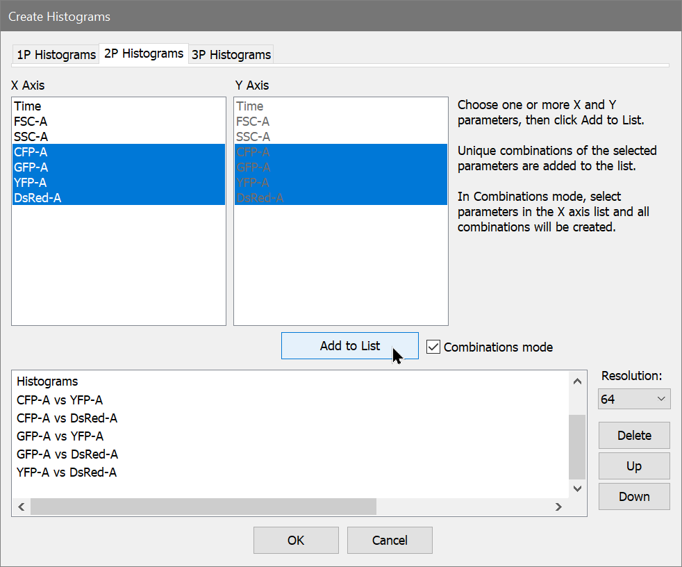
4. In the Create Histograms dialog, select FSC-A in the X Axis list, SSC-A in the Y Axis list, and click Add to List.
5. In the X Axis list, select CFP-A,
GFP-A, YFP-A,
DsRed-A. Enable the Combinations
mode checkbox, and click Add to
List. All combinations of the four fluorochromes will appear in
the histogram list. Click the OK
button.
The program will open the first file and display seven scatter plots. The batch toolbar will appear at the bottom of the application window. We're ready to let WinList determine the correct compensation settings by reading each of the control files.
6. Draw a region around the cells of interest in the FSC-A vs SSC-A plot as shown.
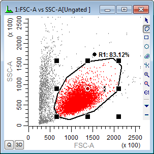
7. Apply this gate to each of the remaining dot plots.
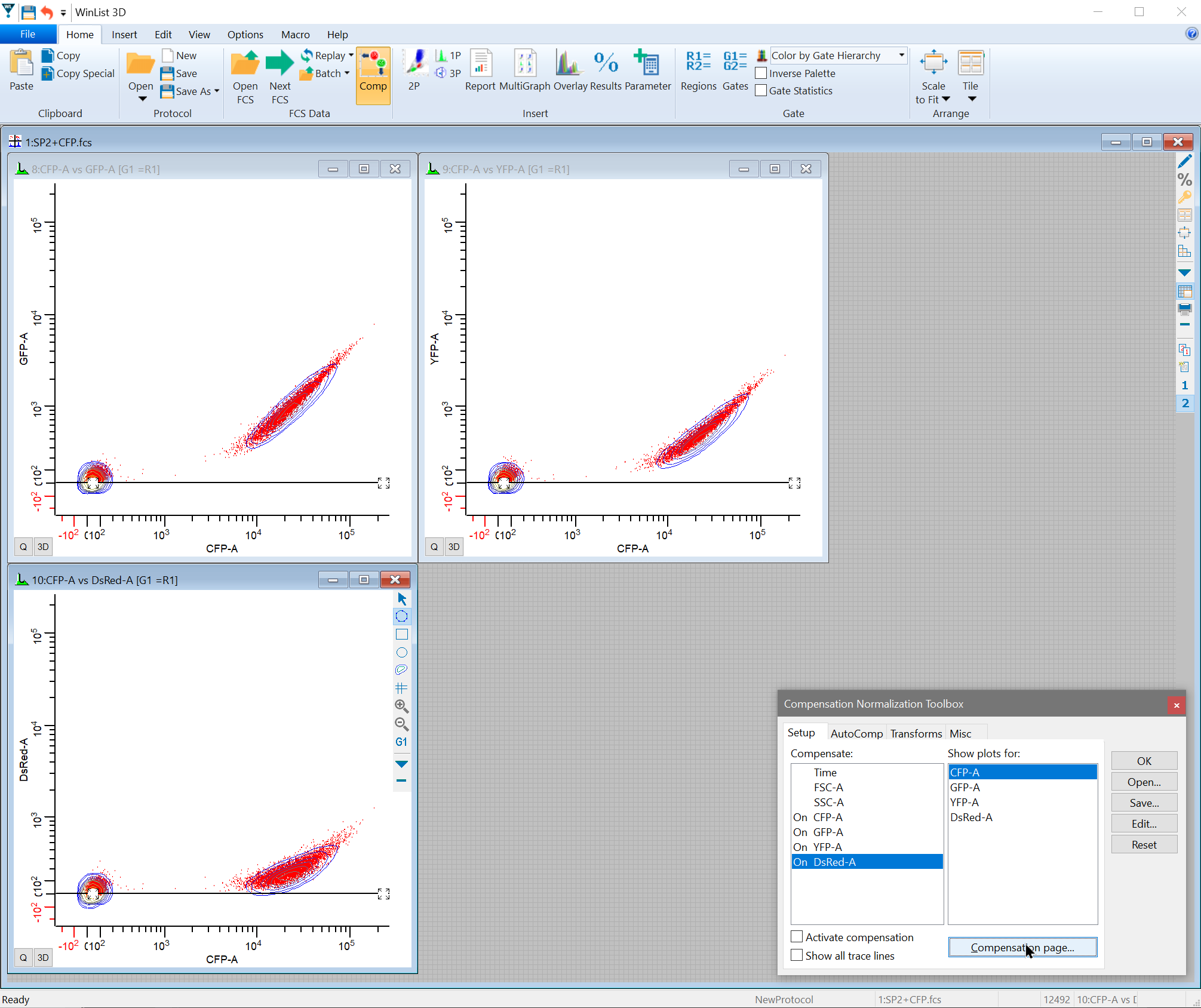
8. Click the Compensation Toolbox button on the ribbon bar. The Compensation Normalization Toolbox will be displayed.

9. In the Compensate listbox, click CFP-A, GFP-A, YFP-A, and DsRed-A measurements to enable them for compensation. Notice the label shows "On" in the listbox, and an entry appears in the Show plots for list for each enabled measurement.
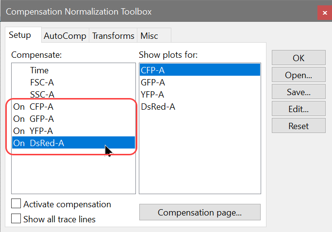
Only enable the parameters that you want to compensate in the Compensate list.
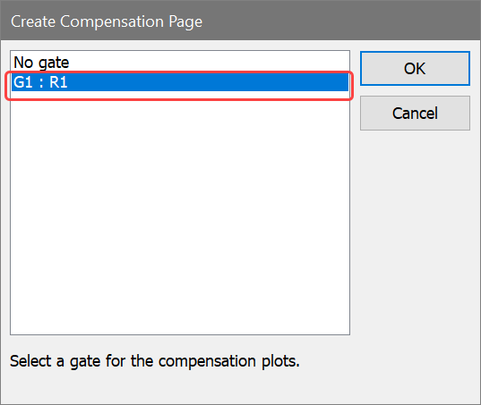
10. Next, click the Compensation page... button to create a page specifically designed for setting up compensation. Use this button any time you want to assign a gate to plots on the Compensation page. A dialog is displayed to select a gate for this page. Choose G1 and click OK.
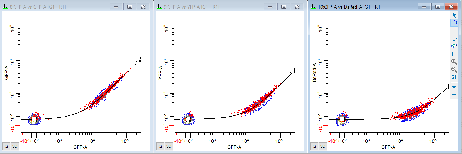
The Compensation page (page 2) is created with three plots showing CFP-A on the X-axis. The Y-axis of each plot shows one of the other compensation measurements. The straight, horizontal lines on the plots are the trace lines. In the next step, WinList will position the trace lines through the centers of the populations.
11. Click
CFP-A
in the Show plots for
listbox, and WinList performs a regression through the events.
It positions the trace lines through the median of the populations.
This is WinList's automatic positioning routine at work.
Manual compensation adjustments
With single-color controls, the program almost always does a better
job of determining the correct slope than we can by eye. If, however,
you need to make an adjustment to the trace lines, this is a simple drag
operation. The square handles that appear at each end of the trace line
are used for this purpose.
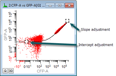
The position of a trace line determines the slope and intercept of a line
through the center of the data. Adjusting the handle in the low-intensity
area sets the intercept, and the slope is determined by the position of
the handle in the high-intensity area. As you move the slope handle toward
the diagonal, you increase the amount of compensation that will be applied
to the data. The intercept handle actually has very little impact on the
compensation.
In rare cases, you may need to apply more compensation than the trace lines normally permit. You can give greater freedom of movement to the trace lines by holding down the Shift key on the keyboard when moving its handles. This allows each trace line handle to move along two sides of the histogram, with slopes of greater than 1.0.
Processing the remaining control files
With the first single-color control all set, let's process the remaining single-color control files.
12. On the batch toolbar at the bottom of the application window, click the Next Batch Item button to read in the next file, SP2+DsRed.fcs. You will see the title in the data source window change to show the new file name.

13. Click the "DsRed-A" in the Show plots for listbox. WinList shows the correct plots for DsRed compensation and automatically positions the trace lines.
14. Click the Next Batch Item button
to read in the next file, SP2+GFP.fcs.
Choose the "GFP-A" from the Show
plots for listbox. Once again, WinList automatically positions
the Trace lines.
15. And once more, click the Next Batch Item button to read in the next file, SP2+YFP.fcs. Choose the "YFP-A" from the Show plots for listbox to tell WinList to position the trace lines.
Applying the compensation
Believe or not, we just finished setting up the compensation! WinList did most of the work for us as each single color control was loaded and we selected the appropriate trace line option. Now that the spill coefficients have been determined for each fluorochrome, we are ready to apply the compensation.
16. Click the Activate compensation checkbox.
Two things will happen. First, the histograms will redraw to display
the compensated data. Secondly, the trace lines will disappear, replaced
with small +
and -
buttons on the histograms. These buttons allow you to adjust the compensation
settings with the compensation system activated. To see all of the adjustment
buttons, enable the Show all trace lines
checkbox.
Let's open a 4-color file and test the compensation settings.
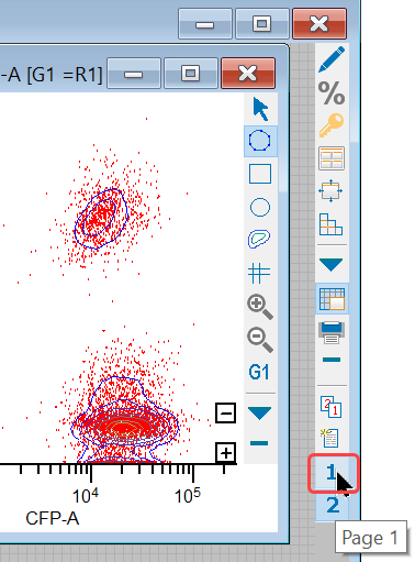
17. On the data source toolbar, click the "1" button to return to page 1.
18. Click the Next FCS File button on the ribbon bar. Choose Mix all.fcs and click Open.

The newly-defined compensation is applied to the data in the new file as
it is read, and we can see well-compensated populations in each plot.
You may have noticed that the log axes on the histograms show values less than zero. WinList supports several log-like transformations that allow negative values to be displayed: HyperLog, Hyperbolic Sine, and VLog. These transforms are log-like, but do not have the limitations of the log transform, in which zero and negative values are undefined.
When compensation is applied to events, it is possible for the value of a parameter to become zero or negative. Color compensation is a subtractive process, and when significant compensation levels are applied to low intensity events, the result is often a negative number - sometimes a large, negative number.
You can toggle between transformations quickly using buttons that appear on the Transforms tab of the Compensation Toolbox. This tab also provides a control to Optimize transforms.
19. Let's save a protocol for this setup so that it can be used in the next tutorial. Click the Save button and name the protocol "CompensationTutorial".
Reset Auto-Compensation
We need to restore your Auto-Compensation preference to its original setting.
20. Choose Options->Preferences, and select the Data Source branch of the Preferences tree. Look for an option named Auto-Compensation and set it to your original setting.
A few more notes
If you want to apply the same compensation to a series of files, you can use the Next File button on the ribbon bar to open each file into the compensated data source window.
Compensation is only active on the data source window that was used to set up the trace lines. Different data source windows can have different compensation settings.
You can also use the compensation system to make adjustments to a previously compensated file. To do this, enable the parameters you want to adjust, select a measurement in the Show plots for list, and make the adjustments. When you are finished, turn on the compensation system by checking the Activate compensation checkbox.
Summary
WinList's N-Color Compensation system is very quick and easy to use. You can use it to compensate any number of fluorescent measurements for signal crossover. This is best accomplished through the use of single-color control files, which are read one at a time to determine the best compensation settings.
Trace lines are graphical elements displayed in the histograms that you are compensating. WinList can automatically position trace lines using a robust fitting algorithm, and it uses the slopes of trace lines to set up a compensation matrix.
See Also: