Purpose:
The purpose of this tutorial is to demonstrate the appropriate use of ModFit LT linearity controls. The goals of the tutorial are listed below.
1. Define linearity and its potential effects on cell cycle analysis.
2. Show an example of a fit with an inappropriate linearity setting.
3. Demonstrate the manual method of adjusting linearity.
4. Discuss the linearity configuration settings.
5. Discuss a recommended approach to modeling with an optimized linearity setting.
Definition and Potential Effects
Linearity, in this discussion, is defined as the observed ratio between the DNA Diploid G2M and G0G1 positions. Theoretically, this value should be 2.0, but it can vary from this ideal value.
Linearity affects cell cycle analysis in several ways. The first effect is that for models that have indistinct G2M peaks, the program uses the linearity setting to position the G2M in the fitting process. For example, if a G1 peak is found at channel 100, the G2M position would be at 200 with the linearity setting of 2.0. If the linearity setting were 1.9, the G2M position would be 190.
The second major effect is on the aggregation model component. This model component assumes, for example, that doublet positions are twice singlet positions and triplet positions are three times the singlet positions. ModFit LT uses the linearity setting to transform the data so that it is perfectly linear prior to creating the theoretical shape of the aggregate distribution. Thus, linearity can also affect the positions of computed aggregates and affect the model fit and S-Phase estimate.
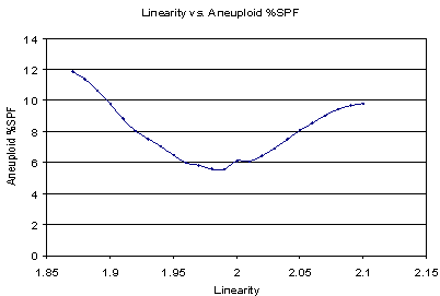
How important is the linearity setting in estimating the S-Phase fraction? It can change S-Phase estimates significantly, as shown in the next graph.

In this particular example, a linearity setting of either 1.90 or 2.1 results in approximately twice the aneuploid S-Phase estimate as a value of 1.99.
Therefore, it is important to optimize this setting for a particular histogram and model in order to obtain accurate and consistent S-Phase estimates.
Example of inappropriate linearity setting
Here is a report demonstrating a model that used an inappropriate linearity setting.
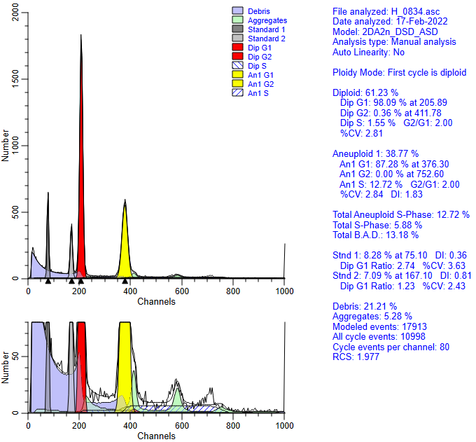
Notice that the Aneuploid S-Phase is quite high and the reduced chi-square is 1.97 for this analysis.
In order to better appreciate the linearity effects, we also show a zoomed view of the graph. This allows us to easily see the Diploid G2M peak and aggregates.
Notice that the diploid G2M model component has disappeared - overwhelmed by the aggregate component.
Automatic linearity detection from Quick Model Editor
Let's use a feature in ModFit LT that is designed to automatically find this optimal linearity setting.
Click the down-arrow on the right of the Fit button on the ribbon bar and choose Auto Linearity to trigger the command.
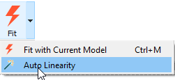
With this method, the program models the data with a set of linearity settings, searching for the one that results in the lowest reduced chi-square. The message status bar in the lower-left corner indicates its progress.
After it has completed this analysis, it re-fits the histogram with the optimized linearity setting. For this example the optimized linear setting is 1.96.
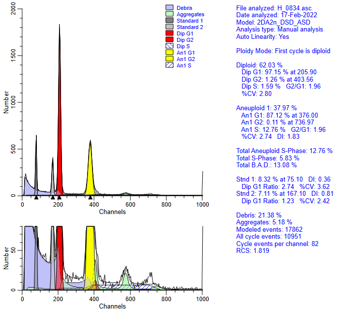
The advantage of using the automatic linearity detection is that it potentially eliminates an important factor in S-Phase estimate variability.
We can also automate the entire process with batch processing.
Automatic linearity adjustment
When you are processing a batch of files in a project, you can enable an option to perform auto-linearity on each sample file. This option is available for Cell Cycle projects.
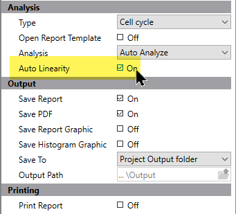
This setting optimizes linearity automatically for each file.
Linearity configuration settings
How does the program determine the starting and ending linearity value to test in the auto linearity detection system? These settings are stored in the Options and Configuration section of the program. This dialog can be displayed if you have administrative access to the program by choosing the Configuration command from the Options tab of the ribbon bar.

ModFit LT contains reasonable default values for these settings. If your laboratory has a smaller range of possible linearity values, you can save considerable time by making the Low linearity and High linearity settings more restrictive.
A recommended approach to modeling with an optimized linearity setting
Our recommended approach to the routine analysis of DNA files is as follows. First, find a good average linearity setting for your laboratory and enter it into the Auto Analysis Settings option in the program. You may also need to tailor other aspects of the auto analysis system as well.
Second, enable Auto Linearity in your Cell Cycle projects to optimize the linearity value for each sample.